Examples
Note
The footnotes in this section provide scientific background to help you understand the motivation and physical meaning of these example calculations. They can be skipped if you are familiar already or aren’t interested in those details.
In this section, we use the example data files included with aospy to demonstrate the standard aospy workflow of executing and submitting multiple calculations at once.
These files contain timeseries of monthly averages of two variables generated by an idealized [1] aquaplanet [2] climate model:
- Precipitation generated through gridbox-scale condensation
- Precipitation generated through the model’s convective parameterization [3]
Using this data that was directly outputted by the model, let’s compute two other useful quantities: (1) the total precipitation rate, and (2) the fraction of the total precipitation rate that comes from the convective parameterization. We’ll compute the time-average over the whole duration of the data, both at each gridpoint and aggregated over specific regions.
Preliminaries
First we’ll save the path to the example data in a local variable, since we’ll be using it in several places below.
In [1]: import os  # Python built-in package for working with the operating system

In [2]: import aospy

In [3]: rootdir = os.path.join(aospy.__path__[0], 'test', 'data', 'netcdf')
Now we’ll use the fantastic xarray package to inspect the data:
In [4]: import xarray as xr

In [5]: xr.open_mfdataset(os.path.join(rootdir, '000[4-6]0101.precip_monthly.nc'),
   ...:                   decode_times=False)
   ...:
Out[5]:
<xarray.Dataset>
Dimensions:            (lat: 64, latb: 65, lon: 128, lonb: 129, nv: 2, time: 36)
Coordinates:
  * lonb               (lonb) float64 -1.406 1.406 4.219 7.031 9.844 12.66 ...
  * lon                (lon) float64 0.0 2.812 5.625 8.438 11.25 14.06 16.88 ...
  * latb               (latb) float64 -90.0 -86.58 -83.76 -80.96 -78.16 ...
  * lat                (lat) float64 -87.86 -85.1 -82.31 -79.53 -76.74 ...
  * nv                 (nv) float64 1.0 2.0
  * time               (time) float64 1.111e+03 1.139e+03 1.17e+03 1.2e+03 ...
Data variables:
    condensation_rain  (time, lat, lon) float64 5.768e-06 5.784e-06 ...
    convection_rain    (time, lat, lon) float64 0.0 0.0 0.0 0.0 0.0 0.0 0.0 ...
    time_bounds        (time, nv) float64 1.095e+03 1.126e+03 1.126e+03 ...
    average_DT         (time) float64 31.0 28.0 31.0 30.0 31.0 30.0 31.0 ...
    zsurf              (time, lat, lon) float64 0.0 0.0 0.0 0.0 0.0 0.0 0.0 ...
We see that, in this particular model, the variable names for these two forms of precipitation are “condensation_rain” and “convection_rain”, respectively. The file also includes the coordinate arrays (“lat”, “time”, etc.) that indicate where in space and time the data refers to.
Now that we know where and what the data is, we’ll proceed through the workflow described in the Using aospy section of this documentation.
Describing your data
Runs and DataLoaders
First we create an aospy.Run object that stores metadata
about this simulation. This includes specifying where its files are
located via an aospy.data_loader.DataLoader object.
DataLoaders specify where your data is located and organized. Several types of DataLoaders exist, each for a different directory and file structure; see the API Reference for details.
For our simple case, where the data comprises a single file, the
simplest DataLoader, a DictDataLoader, works well. It maps your
data based on the time frequency of its output (e.g. 6 hourly, daily,
monthly, annual) to the corresponding netCDF files via a simple
dictionary:
In [6]: from aospy.data_loader import DictDataLoader

In [7]: file_map = {'monthly': os.path.join(rootdir, '000[4-6]0101.precip_monthly.nc')}

In [8]: data_loader = DictDataLoader(file_map)
We then pass this to the aospy.Run constructor, along with
a name for the run and an optional description.
In [9]: from aospy import Run

In [10]: example_run = Run(
   ....:     name='example_run',
   ....:     description='Control simulation of the idealized moist model',
   ....:     data_loader=data_loader
   ....: )
   ....:
Note
See the API reference for other optional arguments for this and the other core aospy objects used in this tutorial.
Models
Next, we create the aospy.Model object that describes the
model in which the simulation was executed. One important attribute
is grid_file_paths, which consists of a sequence (e.g. a tuple or
list) of paths to netCDF files from which physical attributes of that
model can be found that aren’t already embedded in the output netCDF
files.
For example, often the land mask that defines which gridpoints are
ocean or land is outputted to a single, standalone netCDF file, rather
than being included in the other output files. But we often need the
land mask, e.g. to define certain land-only or ocean-only
regions. [4] This and other grid-related properties shared
across all of a Model’s simulations can be found in one or more of the
files in grid_file_paths.
The other important attribute is runs, which is a list of the
aospy.Run objects that pertain to simulations performed in
this particular model.
In [11]: from aospy import Model

In [12]: example_model = Model(
   ....:     name='example_model',
   ....:     grid_file_paths=(
   ....:         os.path.join(rootdir, '00040101.precip_monthly.nc'),
   ....:         os.path.join(rootdir, 'im.landmask.nc')
   ....:     ),
   ....:     runs=[example_run]  # only one Run in our case, but could be more
   ....: )
   ....:
Projects
Finally, we associate the Model object with an
aospy.Proj object. This is the level at which we specify
the directories to which aospy output gets written.
In [13]: from aospy import Proj

In [14]: example_proj = Proj(
   ....:     'example_proj',
   ....:     direc_out='example-output',  # default, netCDF output (always on)
   ....:     tar_direc_out='example-tar-output', # output to .tar files (optional)
   ....:     models=[example_model]  # only one Model in our case, but could be more
   ....: )
   ....:
This extra aospy.Proj level of organization may seem like
overkill for this simple example, but it really comes in handy once
you start using aospy for more than one project.
Defining physical quantities and regions
Having now fully specified the particular data of interest, we now define the general physical quantities of interest and any geographic regions over which to aggregate results.
Physical variables
We’ll first define aospy.Var objects for the two variables
that we saw are directly available as model output:
In [15]: from aospy import Var

In [16]: precip_largescale = Var(
   ....:      name='precip_largescale',  # name used by aospy
   ....:      alt_names=('condensation_rain',),  # its possible name(s) in your data
   ....:      def_time=True,  # whether or not it is defined in time
   ....:      description='Precipitation generated via grid-scale condensation',
   ....:  )
   ....:  precip_convective = Var(
   ....:      name='precip_convective',
   ....:      alt_names=('convection_rain', 'prec_conv'),
   ....:      def_time=True,
   ....:      description='Precipitation generated by convective parameterization',
   ....:  )
   ....:
When it comes time to load data corresponding to either of these from
one or more particular netCDF files, aospy will search for variables
matching either name or any of the names in alt_names,
stopping at the first successful one. This makes the common problem
of model-specific variable names a breeze: if you end up with data
with a new name for your variable, just add it to alt_names.
Warning
This assumes that the name and all alternate names are unique to that variable, i.e. that in none of your data do those names actually signify something else. If that was indeed the case, aospy can potentially grab the wrong data without issuing an error message or warning.
Next, we’ll create functions that compute the total precipitation and
convective precipitation fraction and combine them with the above
aospy.Var objects to define the new aospy.Var
objects:
In [18]: def total_precip(condensation_rain, convection_rain):
   ....:     """Sum of large-scale and convective precipitation."""
   ....:     return condensation_rain + convection_rain
   ....:

In [19]: def conv_precip_frac(precip_largescale, precip_convective):
   ....:     """Fraction of total precip that is from convection parameterization."""
   ....:     total = total_precip(precip_largescale, precip_convective)
   ....:     return precip_convective / total.where(total)
   ....:

In [20]: precip_total = Var(
   ....:     name='precip_total',
   ....:     def_time=True,
   ....:     func=total_precip,
   ....:     variables=(precip_largescale, precip_convective),
   ....: )
   ....:

In [21]: precip_conv_frac = Var(
   ....:    name='precip_conv_frac',
   ....:    def_time=True,
   ....:    func=conv_precip_frac,
   ....:    variables=(precip_largescale, precip_convective),
   ....: )
   ....:
Notice the func and variables attributes that weren’t in the
prior Var constuctors. These signify the function to use and the
physical quantities to pass to that function in order to compute the
quantity.
Note
Although variables is passed a tuple of Var objects
corresponding to the physical quantities passed to func,
func should be a function whose arguments are the
xarray.DataArray objects corresponding to those
variables. aospy uses the Var objects to load the DataArrays
and then passes them to the function.
This enables you to write simple, expressive functions comprising only the physical operations to perform (since the “data wrangling” part has been handled already).
Warning
Order matters in the tuple of aospy.Var objects passed
to the variables attribute: it must match the order of the call
signature of the function passed to func.
E.g. in precip_conv_frac above, if we had mistakenly done
variables=(precip_convective, precip_largescale), the
calculation would execute without error, but all of the results
would be physically wrong.
Geographic regions
Last, we define the geographic regions over which to perform
aggregations and add them to example_proj. We’ll look at the
whole globe and at the Tropics:
In [22]: from aospy import Region

In [23]: globe = Region(
   ....:     name='globe',
   ....:     description='Entire globe',
   ....:     lat_bounds=(-90, 90),
   ....:     lon_bounds=(0, 360),
   ....:     do_land_mask=False
   ....: )
   ....:

In [24]: tropics = Region(
   ....:     name='tropics',
   ....:     description='Global tropics, defined as 30S-30N',
   ....:     lat_bounds=(-30, 30),
   ....:     lon_bounds=(0, 360),
   ....:     do_land_mask=False
   ....: )
   ....:

In [25]: example_proj.regions = [globe, tropics]
We now have all of the needed metadata in place. So let’s start crunching numbers!
Submitting calculations
Using aospy.submit_mult_calcs()
Having put in the legwork above of describing our data and the
physical quantities we wish to compute, we can submit our desired
calculations for execution using aospy.submit_mult_calcs().
Its sole required argument is a dictionary specifying all of the
desired parameter combinations.
In the example below, we import and use the example_obj_lib module
that is included with aospy and whose objects are essentially
identical to the ones we’ve defined above.
In [26]: from aospy.examples import example_obj_lib as lib

In [27]: calc_suite_specs = dict(
   ....:     library=lib,
   ....:     projects=[lib.example_proj],
   ....:     models=[lib.example_model],
   ....:     runs=[lib.example_run],
   ....:     variables=[lib.precip_largescale, lib.precip_convective,
   ....:                lib.precip_total, lib.precip_conv_frac],
   ....:     regions='all',
   ....:     date_ranges='default',
   ....:     output_time_intervals=['ann'],
   ....:     output_time_regional_reductions=['av', 'reg.av'],
   ....:     output_vertical_reductions=[None],
   ....:     input_time_intervals=['monthly'],
   ....:     input_time_datatypes=['ts'],
   ....:     input_time_offsets=[None],
   ....:     input_vertical_datatypes=[False],
   ....: )
   ....:
See the API Reference on aospy.submit_mult_calcs() for more
on calc_suite_specs, including accepted values for each key.
submit_mult_calcs() also accepts a second dictionary
specifying some options regarding how we want aospy to display,
execute, and save our calculations. For the sake of this simple
demonstration, we’ll suppress the prompt to confirm the calculations,
submit them in serial rather than parallel, and suppress writing
backup output to .tar files:
In [28]: calc_exec_options = dict(prompt_verify=False, parallelize=False,
   ....:                          write_to_tar=False)
   ....:
Now let’s submit this for execution:
In [29]: from aospy import submit_mult_calcs

In [30]: calcs = submit_mult_calcs(calc_suite_specs, calc_exec_options)
This permutes over all of the parameter settings in
calc_suite_specs, generating and executing the resulting
calculation. In this case, it will compute all four variables and
perform annual averages, both for each gridpoint and regionally
averaged.
Although we do not show it here, this also prints logging information to the terminal at various steps during each calculation, including the filepaths to the netCDF files written to disk of the results.
Results
The result is a list of aospy.Calc objects, one per
simulation.
In [31]: calcs
Out[31]:
[<aospy.Calc instance: precip_conv_frac, example_proj, example_model, example_run>,
 <aospy.Calc instance: precip_total, example_proj, example_model, example_run>,
 <aospy.Calc instance: precip_convective, example_proj, example_model, example_run>,
 <aospy.Calc instance: precip_largescale, example_proj, example_model, example_run>]
Each aospy.Calc object includes the paths to the output
In [32]: calcs[0].path_out
Out[32]:
{'av': 'example-output/example_proj/example_model/example_run/precip_conv_frac/precip_conv_frac.ann.av.from_monthly_ts.example_model.example_run.0004-0006.nc',
 'reg.av': 'example-output/example_proj/example_model/example_run/precip_conv_frac/precip_conv_frac.ann.reg.av.from_monthly_ts.example_model.example_run.0004-0006.nc'}
and the results of each output type
Note
You may have noticed that subset_... and raw_...
coordinates have years 1678 and later, when our data was from model
years 4 through 6. This is because technical details upstream limit the range of supported whole years to 1678-2262.
As a workaround, aospy pretends that any timeseries that starts before the beginning of this range actually starts at 1678. An upstream fix is currently under way, at which point all dates will be supported without this workaround.
Gridpoint-by-gridpoint
Let’s plot (using matplotlib) the time
average at each gridcell of all four variables. For demonstration
purposes, we’ll load the data that was saved to disk using xarray
rather than getting it directly from the data_out attribute as
above.
In [33]: from matplotlib import pyplot as plt

In [34]: fig = plt.figure()

In [35]: for i, calc in enumerate(calcs):
   ....:     ax = fig.add_subplot(2, 2, i+1)
   ....:     arr = xr.open_dataset(calc.path_out['av']).to_array()
   ....:     if calc.name != precip_conv_frac.name:
   ....:         arr *= 86400  # convert to units mm per day
   ....:     arr.plot(ax=ax)
   ....:     ax.set_title(calc.name)
   ....:     ax.set_xticks(range(0, 361, 60))
   ....:     ax.set_yticks(range(-90, 91, 30))
   ....:

In [36]: plt.tight_layout()

In [37]: plt.show()
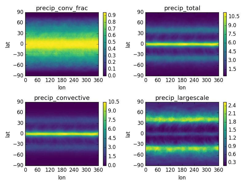
We see that precipitation maximizes at the equator and has a secondary maximum in the mid-latitudes. [5] Also, the convective precipitation dominates the total in the Tropics, but moving poleward the gridscale condensation plays an increasingly larger fractional role (note different colorscales in each panel). [6]
Regional averages
Now let’s examine the regional averages. We find that the global annual mean total precipitation rate for this run (converting to units of mm per day) is:
In [38]: for calc in calcs:
   ....:     ds = xr.open_dataset(calc.path_out['reg.av'])
   ....:     if calc.name != precip_conv_frac.name:
   ....:         ds *= 86400  # convert to units mm/day
   ....:     print(calc.name, ds, '\n')
   ....:
precip_conv_frac <xarray.Dataset>
Dimensions:              ()
Coordinates:
    subset_end_date      datetime64[ns] 1680-12-31
    raw_data_start_date  datetime64[ns] 1678-01-01
    subset_start_date    datetime64[ns] 1678-01-01
    raw_data_end_date    datetime64[ns] 1681-01-01
Data variables:
    globe                float64 0.598
    tropics              float64 0.808

precip_total <xarray.Dataset>
Dimensions:              ()
Coordinates:
    raw_data_end_date    datetime64[ns] 1681-01-01
    raw_data_start_date  datetime64[ns] 1678-01-01
    subset_start_date    datetime64[ns] 1678-01-01
    subset_end_date      datetime64[ns] 1680-12-31
Data variables:
    globe                float64 3.025
    tropics              float64 3.51

precip_convective <xarray.Dataset>
Dimensions:              ()
Coordinates:
    raw_data_end_date    datetime64[ns] 1681-01-01
    raw_data_start_date  datetime64[ns] 1678-01-01
    subset_start_date    datetime64[ns] 1678-01-01
    subset_end_date      datetime64[ns] 1680-12-31
Data variables:
    globe                float64 2.11
    tropics              float64 3.055

precip_largescale <xarray.Dataset>
Dimensions:              ()
Coordinates:
    raw_data_end_date    datetime64[ns] 1681-01-01
    raw_data_start_date  datetime64[ns] 1678-01-01
    subset_start_date    datetime64[ns] 1678-01-01
    subset_end_date      datetime64[ns] 1680-12-31
Data variables:
    globe                float64 0.9149
    tropics              float64 0.4551
As was evident from the plots, we see that most precipitation (80.8%) in the tropics comes from convective rainfall, but averaged over the globe the large-scale condensation is a more equal player (40.2% for large-scale, 59.8% for convective).
Beyond this simple example
Scaling up
In this case, we computed time averages of four variables, both at each gridpoint (which we’ll call 1 calculation) and averaged over two regions, yielding (4 variables)*(1 gridcell operation + (2 regions)*(1 regional operation)) = 12 total calculations executed. Not bad, but 12 calculations is few enough that we probably could have handled them without aospy.
The power of aospy is that, with the infrastructure we’ve put in place, we can now fire off additional calculations at any time. Some examples:
- Set
output_time_regional_reductions=['ts', 'std', 'reg.ts',
'reg.std']
: calculate the timeseries (‘ts’) and standard deviation (‘std’) of annual mean values at each gridpoint and for the regional averages. - Set
output_time_intervals=range(1, 13): average across years for each January (1), each February (2), etc. through December (12). [7]
With these settings, the number of calculations is now (4 variables)*(2 gridcell operations + (2 regions)*(2 regional operations))*(12 temporal averages) = 288 calculations submitted with a single command.
Modifying your object library
We can also add new objects to our object library at any time. For
example, suppose we performed a new simulation in which we modified
the formulation of the convective parameterization. All we would have
to do is create a corresponding aospy.Run object, and then
we can execute calculations for that simulation. And likewise for
models, projects, variables, and regions.
As a real-world example, two of aospy’s developers use aospy for in their own scientific research, with multiple projects each comprising multiple models, simulations, etc. They routinely fire off thousands of calculations at once. And thanks to the highly organized and metadata-rich directory structure and filenames of the aospy output netCDF files, all of the resulting data is easy to find and use.
Example “main” script
Finally, aospy comes included with a “main” script for submitting calculations that is pre-populated with the objects from the example object library. It also comes with in-line instructions on how to use it, whether you want to keep playing with the example library or modify it to use on your own object library.
It is located in “examples” directory of your aospy installation.
Find it via typing python -c "import os, aospy;
print(os.path.join(aospy.__path__[0], 'examples', 'aospy_main.py'))"
from your terminal.
Footnotes
| [1] | An “idealized climate model” is a model that, for the sake of computational efficiency and conceptual simplicity, omits and/or simplifies various processes relative to how they are computed in full, production-class models. The particular model used here is described in Frierson et al 2006. |
| [2] | An “aquaplanet” is simply a climate model in which the the surface is entirely ocean, i.e. there is no land. Interactions between atmospheric and land processes are complicated, and so an aquaplanet avoids those complications while still generating a climate (when zonally averaged, i.e. averaged around each latitude circle) that roughly resembles that of the real Earth’s. |
| [3] | Most climate models generate precipitation through two separate pathways: (1) direct saturation of a whole gridbox, which results in condensation and precipitation, and (2) a “convective parameterization.” The latter simulates the precipitation that, due to subgrid-scale variability, can be expected to occur at some fraction of the area within a gridcell, even though the cell as a whole isn’t saturated. The total precipitation is simply the sum of these “large-scale” and “convective” components. |
| [4] | In this case, the model being used is an aquaplanet, so the mask will be simply all ocean. But this is not generally the case – comprehensive climate and weather models include Earth’s full continental geometry and land topography (at least as well as can be resolved at their particular horizontal grid resolution). |
| [5] | This equatorial rainband is called the Intertropical Convergence Zone, or ITCZ. In this simulation, the imposed solar radiation is fixed at Earth’s annual mean value, which is symmetric about the equator. The ITCZ typically follows the solar radiation maximum, hence its position in this case directly on the equator. |
| [6] | This is a very common result. The gridcells of many climate models are several hundred kilometers by several hundred kilometers in area. In Earth’s Tropics, most rainfall is generated by cumulus towers that are much smaller than this. But in the mid-latitudes, a phenomenon known as baroclinic instability generates much larger eddies that can span several hundred kilometers. |
| [7] | In this particular simulation, the boundary conditions are constant in time, so there is no seasonal cycle. But we could use these monthly averages to confirm that’s actually the case, i.e. that we didn’t accidentally use time-varying solar radiation when we ran the model. |